Measurement and Inference in Wine Tasting
Richard E. Quandt1
Princeton University
The Andrew W. Mellon Foundation
1. Introduction
Numerous situations exist in which a set of judges rates a set of objects.
Common professional situations in which this occurs are certain types of
athletic competitions (figure skating, diving) in which performance is
measured not by the clock but by "form"
and "artistry," and consumer product evaluations, such as those conducted
by Consumer Reports, in which a large number of different brands of
certain items (e.g., gas barbecue grills, air conditioners, etc.) are compared
for performance.2
All of these situations are characterized by the fact that a truly "objective" measure
of quality is missing, and thus quality can be assayed only on the basis of the (subjective) impressions of
judges.
The tasting of wine is, of course, an entirely analogous situation. While there are objective
predictors of the quality of wine,3 which utilize variables such as
sunshine and
rainfall during the growing season, they would be difficult to apply
to a sample of wines representing many small vineyards exposed to identical
weather conditions, such as might be the case in Burgundy, and would not in
any event be able to predict the
impact on wine quality of a faulty cork. Hence, wine tasting is an important
example in which judges rate a set of objects.
In principle, ratings can be either "blind" or "not blind," although it
may be difficult to imagine how a skating competition could be judged without
the judges knowing the identities of the contestants. But whenever possible,
blind ratings are preferable,
because they remove one important aspect of inter-judge variation that
most people would claim is irrelevant, and in fact harmful to the results,
namely "brand loyalty." Thus, wine bottles are typically covered in blind
tastings or wines are decan
ted, and identified only with code names such as A, B, etc.4
But even blind tastings do not remove
all source of unwanted variation. When we ask judges to take a position as
to which wine is best, second best, and so on, we cannot control for the
fact that some people like tannin more than others, or that some are offended
by traces of oxidation more
than others. Another source of variation is that some judge might rate a
wine on the basis of how it tastes now, while another judge rates
the wine on how he or she thinks the wine might taste at its peak.5
Wine tastings can generate data from which we can learn about the
charateristics of both the wines and the judges. In Section 2, we
concentrate on what the ratings of wines can tell us about the wines
themselves, while in Section 3 we deal with what the
ratings can tell us about the judges. Both sets of questions are interesting
and can utilize straightforward statistical procedures.
2. The Rating of Wines
First of all, we note that there is no cardinal measure by which we can
rate wines. Two scales for rating are in common use: (1) the well-known
ordinal rank-scale, by which wines are assigned ranks 1, 2, ...,n,
and (2) a ``grade''-scale, such as the
well-publicized ratings by Robert Parker based on 100 points.6
The grade scale has some of the aspects of a cardinal scale, in that
intervals are interpreted to have
meaning, but is not a cardinal scale in the sense in which the measure
of weights is one.
Ranking Wines. We shall assume that the are m judges and n wines; hence a table of ranks is an m x n table and
for m=4 and n=3 might appear as
Table 1. Rank Table for Judges
                       Judge       Wine ->     A      B       C

                       Orley                   1.     2.      3.
                       Burt                    2.     1.      3.
                       Frank                   1.     3.      2.
                       Richard                 2.     1.      3.

                       Rank Sums               6.     7.     11.
Notice that no tied ranks appear in the table. The organizer of a wine
tasting clearly has a choice of whether tied ranks are or are not permitted.
My colleagues' and my preference is not to permit tied ranks, since tied
ranks encourage "lazy" tasting; when
the sampled wines are relatively similar, the option of using tied ranks
enables the tasters to avoid hard choices. Hence, in what follows, no tied
ranks will appear (except when wines are graded, rather than ranked). What
does the table tell us about
the group's preferences? The best summary measure has to be the rank sums
for the individual wines, which in the present case turn out to be 6, 7,
and 11 respectively. Clearly, wine A appears to be valued most highly and
wine C the least.
The real question is whether one can say that a rank sum is significantly
low or significantly high, since even if judges assign rank sums completely
at random, we would sometimes find that a wine has a very low (high) rank sum.
Kramer computes upper and lower critical values for the rank sums and asserts
that we can test the hypothesis that a wine has a significantly high (low)
rank sum by comparing the actual rank sum with the critical values; if the
rank sum is greater (lower)
than the upper (lower) critical value, the rank sum would be declared
significantly high (low).7 If, in
assigning a rank to a particular wine, each
of m judges chooses exactly one number out of the set (1, 2, ..., n),
the total number of rank patters is nm and it is easy to determine how
many of the possible rank sums are equal to m (the lowest possible rank
sum), ..., and nm (the
highest possible rank sum). From this is easy to determine critical low and
high values such that 5% of the rank sums are lower than the low and 5%
are higher than the high critical value.8
This test is entirely appropriate if one wishes to test {a single rank sum}
for significance.
The problem with the test is that typically one would want to make a statement
about each and every wine in a tasting; hence one would want to compare the
rank sums of all n wines to the critical values; some of the rank sums might
be smaller than the small critical value, some might be larger than the larger of the critical
values, and others might be in-between. Applying the test to each wine, we
would pronounce some of the wines statistically significantly good
(in the tasters' opinion, some
significantly bad, and some not significantly good or bad. Unfortunately,
this is not a valid use of the test. Consider the experiment of judges
assigning ranks to wines one at a time, beginning with wine A. Once a judge
has assigned a particular rank
to that wine, say "1", that rank is no longer available to be assigned by
that judge to another wine. Hence, the remaining rank sums can no longer be
thought to have been generated from the universe of all possible rank sums,
and in fact, the rank sums for the various wines are not independent.
To examine the consequences of applying the Kramer rank sum test to each wine
in a tasting, we resorted to Monte Carlo experiments in which we generated
10,000 random rankings of n wines by m judges; for each of the 10,000
replications we counted the
number of rank sums that were signficantly high and significantly low,
and then classified the replication in a two-way table in which the
(i,j)th entry, (i=0,...,n, j=0,...,n)
indicates the number
of replications in which i rank sums
were significantly low and j rank sums were significantly high. This
experiment was carried out for (m=4, n=4), (m=8, n=8) and (m=8, n=12).
The results are shown in Tables 2, 3, and 4.
Table 2. Number of Significant Rank Sums According to Kramer
for m=4, n=4.
                                            j=
                           i        0        1       2

                           0      6414     1221      0
                           1      1261     1070     16
                           2         0       12      6
Table 3. Number of Significant Rank Sums According to Kramer
for m=8, n=8.
	                                     j=
                         i       0        1       2      3

                         0     4269     1761     93      0
                         1     1774     1532    211      3
                         2       97      192     60      0
                         3        2        3      2      1
Table 4. Number of Significant Rank Sums According to Kramer
for m=8, n=12.
                                       j=
                     i       0       1       2      3      4

                     0     3206    1874    252      4      0
                     1     1915    1627    357     21      1
                     2      245     332    121     11      0
                     3        6      13     12      3      0
Thus, for example, in Table 4, 1,915 out of 10,000 replications had a sole
rank sum that was significantly low by the Kramer criterion, 1,627 replications
had one rank sum that was signficantly low and one rank sum that was
significantly high, 357
replications had one significantly low and two significantly high rank sums,
and so on. It is clear that the Kramer test classifies way too many rank sums
as significant. At the same time, if we apply the Kramer test to a single
(randomly chosen) column
of the rank table, the 10,00 replications give significantly high and low
outcomes as shown in Table 5:
Table 5. Application of Kramer Test to a Single Rank
Sum in Each Replication
                                    Significantly
                           (m,n)     High     Low

                           (4,4)     552      584
                           (8,8)     507      517
                           (8,12)    478      467
While the observed rejection frequencies of the null hypothesis of
"no significant rank sum" are
statistically significantly different from the expected value of 500,
using the normal approximation to the binomial distribution, the numbers are,
at least, "in the ball-park," while in the case of applying the text to
every rank sum in each replication
they are not even near.
This suggests that a somewhat different approach is needed to testing the rank
sums in a given tasting. Each judge's ranks add up to n(n+1)/2 and hence
the sum of the rank sums over all judges is mn(n+1)/2. Hence, denoting the
rank sum for the jth wine by sj,
j=1,...,n, we obtain the sum of the rank sums over j as
SUM sj=mn(n+1)/2,
which, in effect, means that the rank sums for the various wines are located
on an (n-1)-dimensional simplex. The center point of this simplex has
coordinates m(n+1)/2 in every direction, and if every wine had this rank
sum, there would be no difference at all among the
wines. It is plausible that the farther a set of rank sums s1,...,sn
is located from this center, the more pronounced is the departure of
the rankings from the average. However, judging the potential significance
of the departure of a single rank sum from the center point has the same
problem as the Kramer measure.
Therefore we propose to measure the departure of the whole wine tasting
from the average point by the (squared) sum of distances of each rank sum
from the center points, i.e., by
D=SUM(sj-[m(n+1)/2])2.
In order to determine critical values for D, we resorted to Monte Carlo
experiments. Random rank tables were generated for m judges and n wines
(m=4, 5, ..., 12; n=4, 5, ..., 12), and the D-statistic was computed for
each of 10,000 replications;
the critical value of D at the 0.05 level was obtained from the sample
cumulative distributions. These are displayed in Table 6.
Table 6. Critical values for D at the 0.05 level9
                                             n=
                  m   4     5     6     7     8     9     10    11    12

                  4  50    88    140   216   312   430   570   746   954
                  5  60   110    180   278   390   550   716   946  1204
                  6  74   134    218   336   480   664   876  1150  1468
                  7  88   158    256   394   564   780  1036  1344  1712
                  8 102   182    300   452   644   894  1174  1534  1984
                  9 112   206    338   512   732  1014  1342  1742  2236
                 10 122   230    376   580   820  1128  1500  1954  2508
                 11 136   252    420   636   902  1236  1642  2140  2740
                 12 150   276    458   688   992  1360  1836  2358  2998
It is important to keep in mind the correct interpretation of a significant
D-value. Such a value no longer singles out a wine as significantly "good"
or "bad," but singles out an entire set of wines as representing a
significant rank order.
Table 7. Rank Table
                     Judge     Wine ->     A     B     C     D

                     Orley                 1     2     3     4
                     Burt                  2     1     4     3
                     Frank                 3     1     2     4
                     Richard               2     1     4     3

                     Rank Sums             8     5    13    14
The rank sums for the four wines 8, 5, 13, 14, and the Kramer test would say
only that wine D is significantly bad. In the present example,
D=54, and the entire rank order is significant; i.e., B is
significantly better than A, which is significantly better than C,
which is significantly better than D.
A final approach to determining the significance of rank sums is to perform
the Friedman two-way analysis of variance test.10 It tests the hypothesis
that the ranks assigned to the various wines come from the same population. The test statistic is
F=[12/(mn(n+1))]SUMjsj2-3m(n+1)
if there are no ties, and is
F={12SUMjsj2-3m2n(n+1)2}
/mn(n+1)+[mn-SUMiSUMjtaui]tij3/(n-1)}
if there are ties, where taui is the number of sets of tied ranks for
judge i (if there are no ties for judge i, then taui=n) and tij
is the number of items that are tied for judge i in his/her jth
group of tied observations (if there are no ties, tij=1). It is easy to verify that the second
formula reduces to the first if there are no ties. Critical values for small m and
n are given in Siegel and Castellan; for large values F is
distributed under the null hypothesis of no differences among the rank sums
as chi2(n-1). It is clear that the Friedman test and the D-test have
very similar underlying objectives.
Grading Wines. Grading wines consists of assigning "grades" to each wine,
with no restrictions on whether ties are permitted to occur. While the
resulting scale is not a cardinal scale, some meaning does attach to the
level of the numbers assigned to each wine. Thus, if one a 20-point scale, one
judge assigns to three wines the grades 3, 4, 5, while another judge
assigns the grades 18, 19, 20,and a third judge assigns 3, 12, 20, they appear
to be in complete harmony concerning the ranking of wines, but have serious differences of opinion with respect to the
absolute quality. I am somewhat sceptical about the value of the information
contained in such differences. But we always have the option of translating
grades into ranks and then analyzing the ranks with the techniques illustrated above. For this purpose,
we reproduce the grades assigned by 11 judges to 10 wines in a famous 1976
tasting of American and French Bordeaux wines.
Table 8. The Wines in the 1976 Tasting
                 Wine      Name                          Final Rank

                  A    Stag's Leap 1973                     1st
                  B    Ch. Mouton Rothschild 1970           3rd
                  C    Ch. Montrose 1970                    2nd
                  D    Ch. Haut Brion 1970                  4th
                  E    Ridge Mt.Bello 1971                  5th
                  F    Léoville-las-Cases 1971              7th
                  G    Heitz Marthas Vineyard 1970          6th
                  H    Clos du Val 1972                    10th
                  I    Mayacamas 1971                       9th
                  J    Freemark Abbey 1969                  8th
Table 9 contains the judges' grades and Table 10 the conversion of those
grades into ranks. Since grading permits ties, the ranks into which the
grades are converted also have to reflect ties; thus, for example, if
the top two wines were to be tied in a judge's estimation, they would both be assigned a rank of 1.5. Also note that grades and ranks are inversely related: the higher a grade, the better the wine, and hence the lower its rank position.
If we apply the critical values as recommended by Kramer, we would find that
wines A, B, and C are significantly good (in the opinion of the judges) and
wine H is significantly bad. The value of the D-statistic is 2,637, which
is significant for 11 judges and 10 wines according to Table 6, and hence the
entire rank order may be considered significant. Computing the Friedman
two-way analysis of variance test yields a chi2 value of 23.93, which
is significant at the 1 percent level. Hence, the two tests are entirely
compatible and the Friedman test rejects the hypothesis that the medians
of the distributions of the rank sums are the same for the different wines.
In this section we compared several ways of evaluating the significance of
rank sums. In particular, we argued that the D-statistic and the Friedman
two-way analysis of variance tests are more appropriate than the Kramer
statistic, although for the 1976 tasting they basically agree with one another.
Table 9. The Judges's Grades
Wine
Judge A B C D E F G H I J
Pierre Brejoux 14.0 16.0 12.0 17.0 13.0 10.0 12.0 14.0 5.0 7.0
A. D. Villaine 15.0 14.0 16.0 15.0 9.0 10.0 7.0 5.0 12.0 7.0
Michel Dovaz 10.0 15.0 11.0 12.0 12.0 10.0 11.5 11.0 8.0 15.0
Pat. Gallagher 14.0 15.0 14.0 12.0 16.0 14.0 17.0 13.0 9.0 15.0
Odette Kahn 15.0 12.0 12.0 12.0 7.0 12.0 2.0 2.0 13.0 5.0
Ch. Millau 16.0 16.0 17.0 13.5 7.0 11.0 8.0 9.0 9.5 9.0
Raymond Oliver 14.0 12.0 14.0 10.0 12.0 12.0 10.0 10.0 14.0 8.0
Steven Spurrier 14.0 14.0 14.0 8.0 14.0 12.0 13.0 11.0 9.0 13.0
Pierre Tari 13.0 11.0 14.0 14.0 17.0 12.0 15.0 13.0 12.0 14.0
Ch. Vanneque 16.5 16.0 11.0 17.0 15.5 8.0 10.0 16.5 3.0 6.0
J.C. Vrinat 14.0 14.0 15.0 15.0 11.0 12.0 9.0 7.0 13.0 7.0
Table 10. Conversion of Grades into Ranks
                                                    Wine
          Judge             A     B     C     D     E     F     G     H     I     J

          Pierre Brejoux   3.5   2.0   6.5   1.0   5.0   8.0   6.5   3.5  10.0   9.0
          A. D. Villaine   2.5   4.0   1.0   2.5   7.0   6.0   8.5  10.0   5.0   8.5
          Michel Dovaz     8.5   1.5   6.5   3.5   3.5   8.5   5.0   6.5  10.0   1.5
          Pat. Gallagher   6.0   3.5   6.0   9.0   2.0   6.0   1.0   8.0  10.0   3.5
          Odette Kahn      1.0   4.5   4.5   4.5   7.0   4.5   9.5   9.5   2.0   8.0
          Ch. Millau       2.5   2.5   1.0   4.0  10.0   5.0   9.0   7.5   6.0   7.5
          Raymond Oliver   2.0   5.0   2.0   8.0   5.0   5.0   8.0   8.0   2.0  10.0
          Stev. Spurrier   2.5   2.5   2.5  10.0   2.5   7.0   5.5   8.0   9.0   5.5
          Pierre Tari      6.5  10.0   4.0   4.0   1.0   8.5   2.0   6.5   8.5   4.0
          Ch. Vanneque     2.5   4.0   6.0   1.0   5.0   8.0   7.0   2.5  10.0   9.0
          J.C. Vrinat      3.5   3.5   1.5   1.5   7.0   6.0   8.0   9.5   5.0   9.5

          Rank Totals     41.0  43.0  41.5  49.0  55.0  72.5  70.0  79.5  77.5  76.0
          Group Ranking    1     3     2     4     5     7     6    10     9     8
3. Agreement or Disagreement Among the Judges
There are at least two questions we may ask about the similarity or
dissimilarity of the judges' rankings (or grades). The first one concerns
the extent to which the group of judges as a whole ranks (or grades) the
wines similarly. The second one concerns the extent of the correlation is
between a particular pair of judges.
The natural test for the overall concordance among the judges' ratings is
the Kendall W coefficient of concordance.11 It is computed as
W=SUMi(ri -r)2/[n(n2-1)/12]
where ri is the average rank assigned to the ith wine and r is the average of
the averages. Siegel and Castellan again provide tables for testing
the null hypothesis of no concordance for small values of m and n; for
large values,m(n-1)W is approximately distributed as chi2(n-1). In the
case of the wine tasting depicted in Tables 9 and 10, W=0.2417 and the
probability of obtaining a value this high or higher is 0.0059, a highly
significant result showing strong agreement among the judges.
The pairwise correlations between the judges can be assessed by using
either Spearman's rho and Kendall's tau.12 Spearman's rho
is simply the ordinary product-moment correlation based on variables
expressed as ranks, and thus has the standard interpretation of a
correlation coefficient. The philosophy underlying the computation of tau
is quite different. Assume that we have two rankings given by r1 and r2,
where these are n-vectors of rankings by two individuals. To compute tau,
we first sort r1 into natural order and parallel-sort r2 (i.e., ensure that the
ith elements of r1 and r2 both migrate to the same position in their
respective vectors). We then count up the number of instances
in which in r2 a higher rank follows a lower rank (i.e., are in
natural order) and the number of instances in which in r2 a
higher rank precedes a lower rank (reverse order). tau is then
tau=(Number of natural order pairs - Number of reverse order pairs)/[n!/(n-2)!2!]
Clearly, rho and tau can be quite different and it does not make sense
to compare them. In fact, for n=6, the maximal absolute difference rho-tau
can be as large as 0.3882 and the cumulative distributions of rho and tau
obtained by calculating their values for all possible permutations of
ranks appear to be quite different. Since the interpretation of tau
is a little less natural, I prefer to use rho, but from the point of
view of significance testing it does not make a difference which is used; in
fact, Siegel and Catellan point out that the relation between rho and tau
is governed by the inequalities -1<=3tau-2rho<= 1.
A final calculation that may be amusing, even though its statistical
assessment is not entirely clear, is to calculate the correlation between
the rankings of a given judge with the average ranking of the remaining
judges.13 To accomplish this, we must first average the rankings of the remaining
judges and then find the correlation between this average ranking and the ranking of the
given judge. Obviously, repeating this calculation for each of the n judges
gives us n rhos that are not independent of one another, and hence the
significance testing of these n correlations is unclear. But it is an
amusing addendum to a wine tasting, since it gives us some insight as to
who agrees most with "the rest of the herd" (or, conversely, who is the
dominant person with whom the ``herd'' agrees) and who is the real
contrarian. In the case of the1976 wine tasting, the table of correlations
is as follows:
Table 11. Correlation of Each Judge with Rest of Group
                            Judge          Spearman's rho

                            Pierre Brejoux          0.4634
                            A. D. Villaine          0.6951
                            Michel Dovaz           -0.0675
                            Pat. Gallagher         -0.0862
                            Odette Kahn             0.2926
                            Ch. Millau              0.6104
                            Raymond Oliver          0.2455
                            Stev. Spurrier          0.4688
                            Pierre Tari            -0.1543
                            Ch. Vanneque            0.4195
                            J.C. Vrinat             0.6534
4. The Identification of Wines
One aspect of wine tasting that can be both satisfying and challenging is
to ask the judges to try to identify the wines. By identification we do not,
of course, mean that the judges would have to identify the wines out of the
entire universe of all possible wines. It is clear that judges have to be
given some clue concerning the general category of the wines they are drinking,
otherwise it is quite likely that no useful results will be obtained from the
identification exercise, unless the judges are truly great experts.
There are at least two possibilities. The first one is that the judges
have to associate with each actual wine name the appropriate code letter
(A, B, C, etc.) that appears on a bottle. In this case, we continue to
adopt the convention that at the beginning of the tasting the judges are
presented with a list of the wines to be tasted (presumably in alphabetical
order, lest the order of the wines in the list create a presumption that
the first wine is wine A, the second wine B, and so on). Thus, if eight wines
are to be tasted, the task of the judges is to match the actual wine names
with the letters A, B, C, etc. The question we shall investigate is how
we can test the hypothesis that that the identification pattern selected
by a judge is no better than what would be obtained by a chance assignment.
The second possibility is that the judges are not given the names of the
wines but are given their "type" or the type of grape out of which they are
made. Thus, for example, one could have a tasting of cabernet sauvignons from
Bordeaux together with cabernet sauvignons from California (as in the 1976
tasting discussed in the previous section), or one could have a tasting of
Burgundy pinot noirs, together with Oregon pinot noirs and South African
pinot noirs from the Franschoek or Stellenbosch area. The judges would
merely be told the number of wines of each type in the tasting, and their
task is to identify which of wines A, B, C, etc. is a Bordeaux
wine and which a California wine.
Guessing the Name of Each Wine. Consider the case in which n
wines are being tested and let P be an n by n matrix,
the rows of which correspond to the "artificial" names of the wines
(A, B,...) and the columns of which correspond to the actual
names of the wines. We will say that the label in row i is assigned to
(matched with) the label in column j if the element aij=1 and is not
assigned to the label in column j if aij=0. It is obvious that the matrix
P is a valid identification matrix if and only if (1) each row has
exactly one 1 in it and n-1 0s, and (2) each column has exactly
one 1 in it and n-1 0s. Under these circumstances, an identification matrix is
a permutation matrix, i.e., it is a matrix that can be obtained from an identify
matrix by permuting its rows. Obviously, the "truth" can also be represented
by a permutation matrix; its ijth element is 1 if an only if artificial
label i actually corresponds to real label j. This permutation matrix
will be denoted by T.
To measure the extent to which a person's wine identification (as given by
his or her P matrix) corresponds to the truth (the T matrix), we
propose the following measure C:
C=tr(PT)/n
where n is the number of wines, which is just the percentage of wines correctly
identified. The justification for this measure emerges from the following
considerations.
First note that every permutation matrix is its own inverse; i.e.,
P=P-1. The reason is that if we interchange the ith and jth
rows of an identity matrix and then premultiply a given matrix by it, that will have the
effect of interchanging in the given matrix the same pair of rows. Hence, premultiplying
the matrix P by itself, interchanges those rows in P , yielding an
identity matrix for the product. Thus, if a person's P matrix is identical to T, PT is an
identity matrix, the trace of which is equal to n; hence C=1.0 in the case
in which a person identifies each wine correctly. Moreover, C is monotone in the
number of wines correctly identified and if no wines are correctly identified, C=0.
Therefore, in order to judge whether the observed value of C is significant (under t
he null hypothesis of random identification by the judge), we require the sampling
distribution of C.
The are n! permutation matrices, and any one of these matrices P can be paired
with any one of n! possible matrices T, which suggests a formidable number of possible
outcomes. However, the possible outcomes are identical for each of the
possible T matrices; hence without any loss of generality, we may fix T
as the identity matrix. Then PT=P and to compute C it is sufficient to count up how many
of the possible n! P matrices have trace equal to 0, 1, ...
To find the sampling distribution of the trace is formally identical
with the following problem. Let there be n urns, labelled A, B, C, etc,
and let there be n balls, labelled similarly. We shall
randomly place one ball in each urn; we then ask what the probability is
that exactly k of the urns contain a ball that has the same label as
the urn.
It is obvious that the total possible ways in which balls can placed in
urns is n!. It is also obvious that there is exactly one way (out of
n! ways) that every ball is in the urn with the same label, and it is
also obvious that it is impossible for exatly n-1 balls to be in the
like-labelled urn (since if n-1 balls are, then the last one must also be
in a like-labelled urn).
Denote by M(i,j) the number of ways in which you can place j balls
in j urns so that exactly i balls are in like-labelled urns.14
As long as i is not equal to j-1, having exactly i
balls in the like-labelled urns can be done in j!/i!(j-i)! ways. The
remaining urns and balls should produce no match if we want exactly i matches; the
number of ways that that can occur is, by definition, M(0,j-i). The
total number of ways then is M(i,j)=[j!/i!(j-i)!]M(0,j-i). For a value
of n, the totality of outcomes is given by
                            M(n,n)    = 1,
                            M(n-1,n)  = 0,
                            M(n-2,n)  = [n!/2!(n-2)!]M(0,2),
                            M(n-3,n)  = [n!/3!(n-3)!]M(0,3),
                                  .........
                            M(1,n)    = nM(0,n-1),
                            M(0,n)    = n!-SUMjnM(j,n)
The M(i,n) are easily computed because the above equations provide a
simple recursive scheme for the calculations. We obtain the probability
of i matches, i=0,...,n with n urns by dividing each
M(i,n) by n!. These probabilities are shown in Table 12.
Table 12. Sampling Distribution of Trace
                                          trace=
          n     0       1       2       3       4       5       6       7       8

          4    0.375   0.333   0.250   0.000   0.042
          5    0.367   0.375   0.167   0.083   0.000   0.008
          6    0.368   0.367   0.188   0.056   0.021   0.000   0.001
          7    0.368   0.368   0.183   0.062   0.014   0.004   0.001   0.000
          8    0.368   0.368   0.184   0.061   0.016   0.003   0.000   0.000   0.000
          9    0.368   0.368   0.184   0.061   0.015   0.003   0.000   0.000   0.000
          10   0.368   0.368   0.184   0.061   0.015   0.003   0.000   0.000   0.000
          11   0.368   0.368   0.184   0.061   0.015   0.003   0.000   0.000   0.000
          12   0.368   0.368   0.184   0.061   0.015   0.003   0.000   0.000   0.000
It is clear that irrespective of the number n of wines, a trace of 4
or more is a highly significant result and a trace in excess of 2 is still
significant at the 0.1 level of significance. It is also remarkable that
the distribution converges very rapidly in n to a limiting form.
The other question that is of interest is whether the judges, as a whole,
tend to agree or tend not to agree with one another with respect to wine
identification. Here we propose the following measure of the degree of
agreement among the judges.
Let m be the number of judges and denote their identification matrices by
Pi, i=1,...,n. Let Q=SUMinPi and let qij be the typical element of
Q. Since the sum of the elements of each Pi is exactly n, if
there m judges, the mean value of each element of Q is mn/n2=m/n. We
propose as the measure of concordance the variance of the elements of Q,
i.e.,
V=[1/n2]SUMin[qij-(m/n)]2
If all the judges pick the same permutation matrix, n of
the elements of Q will be equal to m and the remaining ones will be zero.
In that case the variance over the elements of Q is
V=[1/n2][n(m-(m/n))2+n(n-1)(m/n)2]=m2(n-1)/n2
If the judges predominantly pick P matrices that are very different, the elements of
Q will be relatively more similar and the variance will be small. In order
to determine what level of variance is significant, we have to determine
the sampling distribution of the variance under the null hypothesis that
the judges pick P matrices at random.
The sampling distributions were determined for the number of wines i, i=4,...,12 and the number of
judges j, j=4,...,15 by Monte Carlo experiments. An experiment
for given i and j consisted of picking j out of the i! permutation matrices
and then computing V as shown above. Each experiment was replicated
10,000 times. Table 13 contains the 10 percent and Table 14 the 5 percent
significance levels for V.
Table 13. 10 Percent Significance Levels for V
                                             m=
         n    4     5     6     7     8     9     10    11    12    13    14    15
          4  1.12  1.44  1.75  2.06  2.38  2.69  3.00  3.31  3.62  3.94  4.25  4.56
          5  1.88  1.12  1.36  1.60  1.84  2.08  2.32  2.56  2.80  3.04  3.28  3.52
          6  0.72  0.92  1.11  1.31  1.50  1.69  1.89  2.08  2.28  2.44  2.67  2.81
          7  0.61  0.78  0.94  1.10  1.26  1.43  1.59  1.76  1.92  2.08  2.24  2.41
          8  0.53  0.67  0.81  0.95  1.09  1.23  1.38  1.52  1.62  1.80  1.91  2.08
          9  0.46  0.59  0.72  0.84  0.96  1.09  1.21  1.33  1.46  1.58  1.68  1.80
         10  0.42  0.53  0.64  0.75  0.86  0.97  1.08  1.17  1.30  1.41  1.52  1.63
         11  0.38  0.48  0.58  0.68  0.78  0.88  0.98  1.07  1.17  1.26  1.37  1.46
         12  0.34  0.44  0.53  0.62  0.71  0.80  0.89  0.98  1.07  1.15  1.25  1.34
Table 14. 5 Percent Significance Levels for V
                                              m=
         n    4     5     6     7     8     9     10    11    12    13    14    15
          4  1.25  1.69  2.00  2.31  2.75  3.06  3.38  3.81  4.12  4.56  4.75  5.19
          5  0.96  1.28  1.52  1.76  2.08  2.32  2.56  2.80  3.12  3.36  3.68  3.92
          6  0.78  1.03  1.22  1.41  1.67  1.81  2.06  2.26  2.50  2.64  2.89  3.08
          7  0.65  0.82  1.02  1.18  1.39  1.55  1.71  1.88  2.04  2.24  2.41  2.57
          8  0.56  0.67  0.81  1.02  1.16  1.33  1.47  1.61  1.75  1.92  2.06  2.20
          9  0.49  0.64  0.76  0.89  1.02  1.16  1.28  1.40  1.53  1.68  1.80  1.93
         10  0.44  0.57  0.68  0.79  0.90  1.01  1.14  1.25  1.36  1.49  1.60  1.71
         11  0.40  0.51  0.61  0.71  0.81  0.93  1.02  1.12  1.22  1.32  1.44  1.54
         12  0.35  0.47  0.56  0.64  0.74  0.83  0.93  1.02  1.11  1.20  1.31  1.40
Identifying Types of Wines.We assume, in
conformity with previous assumptions, that judges are informed of how many
wines of Type I and how many of Type II are present in the sample to be
tasted.15 Before we present tables of the distributions of the number
correctly identified under the null of random assignements, consider the
following example. Let us assume that there are nine wines in all, four of
which are of type X and five of which are of type Y and let us depict
the "true" pattern in the sample as
X X X X Y Y Y Y Y
Now imagine that a particular judge guesses the pattern to be
X X X Y X Y Y Y Y
In that case, he/she will have identified the types of seven wines correctly.
In how many ways can this occur? Making two mistakes implies that one
X-type wine is identified as a Y and one Y-type wine is identified as an
X. In the present case you can choose the X which will be misidentified 4!/1!3! ways and
the Y which will be misidentified as an X in 5!/1!4! ways, for a total of 20 ways.
Can you have exactly six or eight wines identified correctly? The answer
is that there are no ways in which you can have six or eight correct
identifications: for example, to reduce the number of correct identifications,
an additional X must be identified as a Y; but that means that an additional
Y will also be identified as an X, hence if seven correct identifications
is possible, then neither six nor eight will ever be possible. In fact,
since if there are n wines, with n1 of type X and n2 of type Y, n correct
identifications is always a possible outcome, the number of possible correct
identifications is n, n-2, n-4, with the last term in the series for
possible correct number of identifications being n-2min(n1,n2).
We display the distributions for the number of wines correctly
identified for selected values of n1 and n2 in Table 15.
Table 15. Probabilities for the Number of Correctly Identified Wines
n1=4 n1=4 n1=4 n1=5 n1=5 n1=6
n2=4 n2=5 n2=6 n2=5 n2=6 n2=6
Number Probabilities
0 0.014 0. 0. 0.004 0. 0.001
1 0. 0.040 0. 0. 0.013 0.
2 0.229 0. 0.071 0.099 0. 0.039
3 0. 0.317 0. 0. 0.162 0.
4 0.514 0. 0.381 0.397 0. 0.244
5 0. 0.476 0. 0. 0.433 0.
6 0.229 0. 0.429 0.397 0. 0.433
7 0. 0.159 0. 0. 0.325 0.
8 0.014 0. 0.114 0.099 0. 0.244
9 0. 0.008 0. 0. 0.065 0.
10 0. 0. 0.005 0.004 0. 0.039
11 0. 0. 0. 0. 0.002 0.
12 0. 0. 0. 0. 0. 0.001
It is easily seen that there generally does not exist a clear-cut critical
value for the number of correctly identified wines at the 5 percent or 10
percent level, because of the discreteness of the distributions. So, for
example, if n1=4 and n2=5, 7 or more correctly identified wines mean
that randomness is rejected at the 0.167 level. Eight or more correctly
identified wines reject the randomness hypothesis at roughly the 0.1 level
for the next two columns, nine (respectively ten) reject randomness at
roughtly the .05 level for the last two columns.
The last case we consider is the one in which there are three types of
wines, which we label with X, Y, and Z. The situation is quite different in
this case, although two facts remain true: (1) there is exactly one way in
which the number of correct identifications can be equal to the number of wines
n, and (2) there is no way in which exactly n-1 wines are correctly
identified. But it is no longer the case that the number of correct
identifications is either always an even number or always an odd number. Consider
the "true" pattern
X X Y Y Y Z Z Z
The judge's following potential identification patterns produce, respectively,
0, 1, 2, 3, 4, 5, 6, and 8 correct identifications:
>
Y Y Z Z Z X X Y
Y Z Z Z Y X X Y
X X Z Z Z Y Y Y
X Y Z Z Y Y Z X
X X Y Z Z Z Y Y
X Y Y Y Z X Z Z
X Y Y Y X Z Z Z
X X Y Y Y Z Z Z
For a few selected values of n1, n2, n3
we display the probability distributions in Table 16.
Table 16. Probabilities for the Number of Correctly Identified Wines
n1=2 n1=3 n1=3 n1=3
n2=3 n2=3 n2=3 n2=3
n3=3 n3=3 n3=4 n3=5
Number Probability
0 0.043 0.033 0.019 0.006
1 0.150 0.129 0.088 0.049
2 0.259 0.225 0.190 0.139
3 0.257 0.259 0.246 0.224
4 0.188 0.193 0.225 0.237
5 0.064 0.112 0.137 0.187
6 0. 0.032 0.071 0.097
7 0.002 0. 0.017 0.046
8 0. 0.001 0.008 0.010
9 0. 0. 0. 0.004
10 0. 0. 0.000 0.
11 0. 0. 0. 0.000
Thus, with three wines of type X, three of type Y and five of type Z, one
needs at least seven correct identifications in order to assert at
approximately the 0.05 level that the result is significantly better than random.
A final question is how the critical value depends on how many types of
wines there are in a tasting. There is obviously no straightforward answer,
because there are two many things that can vary: the total number of wines,
the number of types of wines, and the number of wines within each type.
But consider a simplified experiment in which we fix the total number of
wines at some power of 2; say 27=128. We could then consider, alternately,
2 types of wines with 64 wines of each type, or 4 types with 32 wines of
each type, or 8 types with 16 wines each, 16 types with 8 wines each, 32
types of 4 wines each, and finally 64 types of 2 wines each. It is
intuitively obvious that if we guess randomly, we will tend to score the
highest degree of correct identification in the first case and the lowest
in the last. For imagine that in the first case we arbitrarily identify
the first 64 wines as type X and the last 64 as type Y. If the order in
which the wines have been arranged is random, we shall correctly identify
on the average 64 of the 128 wines. In the last case, when there are 64
types of 2 wines each, the average number of identifications will be
much smaller. To look at this in another way, in the first case there
is only a single outcome in which no wine is correctly identified (i.e.,
the outcome in which the judge guesses the first 64 wines to be of type X,
whereas they are all of type Y, but in the last case there is a huge
number of possible outcomes in which no wine is correctly identified. We
would therefore expect that as the number of types of wine in the tasting
declines (with the number of wines in each type increasing), the critical
value above which we reject the null hypothesis of randomness in the
identification has to increase.
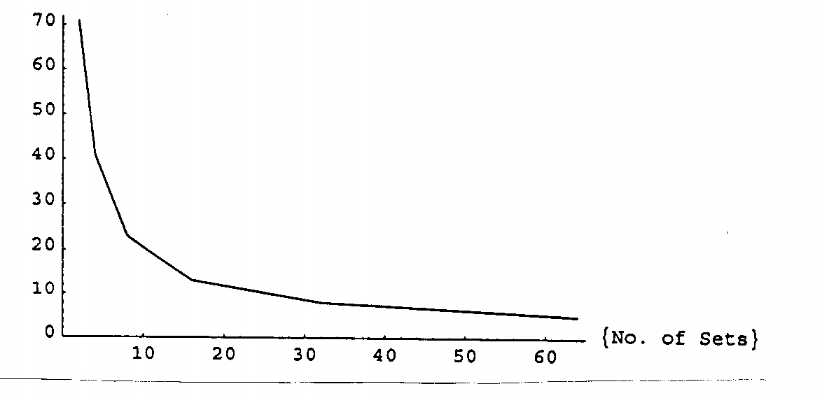
This in fact is the case and we display the dependence of the 5% critical
value in Figure 1. The relation between the critical value and the number
of types of wine is well approximated by a rectangular hyperbola with a
horizontal asymptote of 4.52, which agrees well with what we would expect
from Table 12.16
Figure 1. Critical Values as a Function of the Number of Types
Crit.value
5. Concluding Comments
In this paper, we considered three types of questions: (1) How do we
use the rankings of wines by a set of judges to determine whether some
wines are perceived to be significantly good or bad, (2) How do we judge
the strength of the (various possible) correlations among the judges'
rankings, and (3) How do we determine whether the judges are able to
identify the wines or the types of wines significantly better than would
occur by chance alone. We are able to find appropriate techniques for each
of these questions, and their application is likely to yield considerable
insights into what happens in a blind tasting of wines.
Return to Front Page